Road Marking Training Case Tutorial

Steps

1.Prepare Data

1) Classification

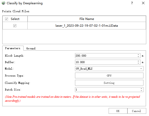
Open the .LiData format point cloud file, and first click the Deep Learning Classification button on the Classification page.

Use the GV_Road_MLS model to classify the point cloud.

2) Generate Intensity Map

For a detailed introduction to this function, refer to Generate Intensity Map.

On the toolbox page, select Map Elements -> Generate Intensity Map.

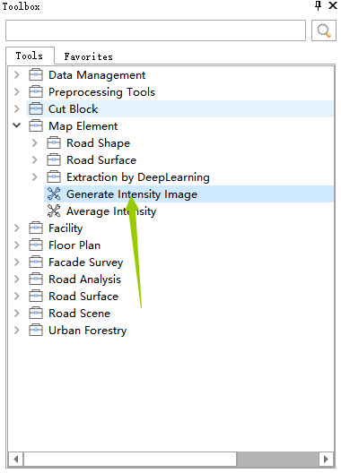
Double-click to open

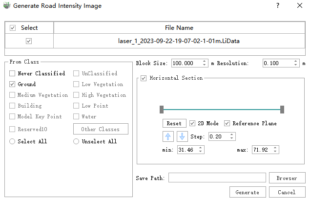
Select ground points on the left source category, set the save path, set the resolution to 0.02m, and click the Generate button.

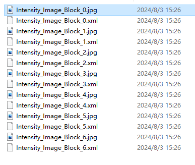
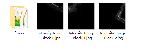
3) Repeat the above steps to generate intensity maps for multiple point clouds, as shown below.

2.Annotate Data

1) Determine Annotation Categories

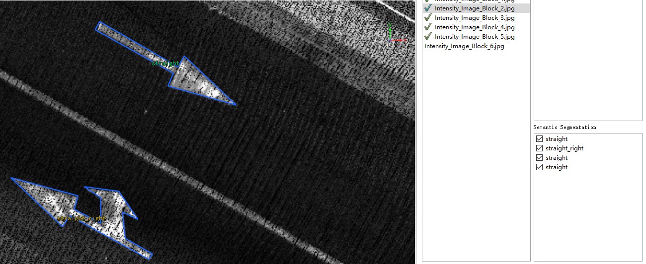
First, determine the types of road signs to be processed. Here, Straight and Straight Right signs are used as examples.

2)Start Annotation

Use the Labeling Tool to annotate the data.

Click the Start Labeling button to open the annotation function, then click the Open Dir button to open the prepared image data.

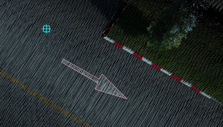
Click the Create Rectangle button to mark the key points of the sign in the image. These key points must be arranged counterclockwise, and each category should have the same number of key points, with the start and end points consistent, as shown below:

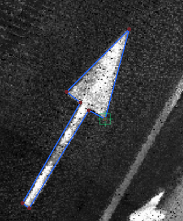
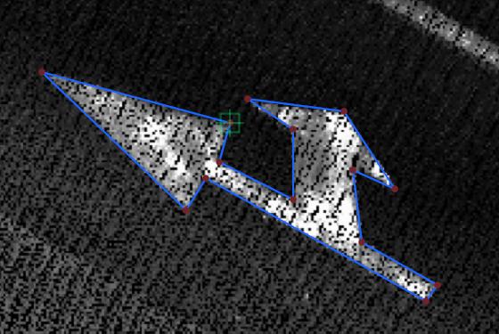
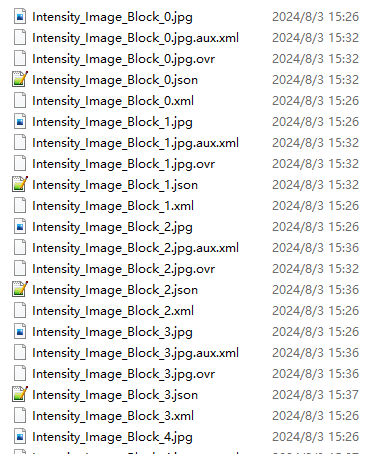
After marking the Straight and Straight Right Turn signs in all prepared images, the resulting data should look like this. (Ensure each type of sign has at least three annotations)

3.Training

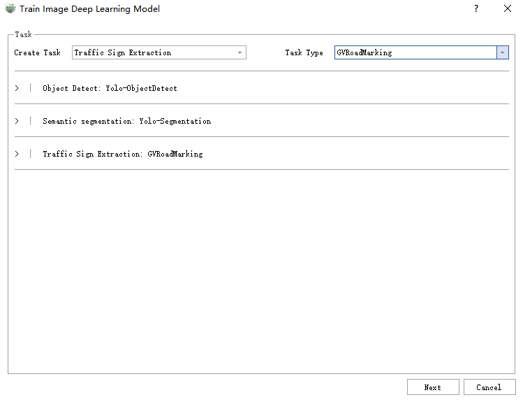
1) Click Raster -> Train Image Deep Learning Model. Since this task involves road sign extraction, select the GVRoadMarking model for semantic segmentation.

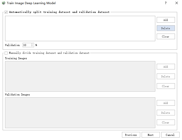
2) Click Next, and choose Automatically split training and validation datasets.

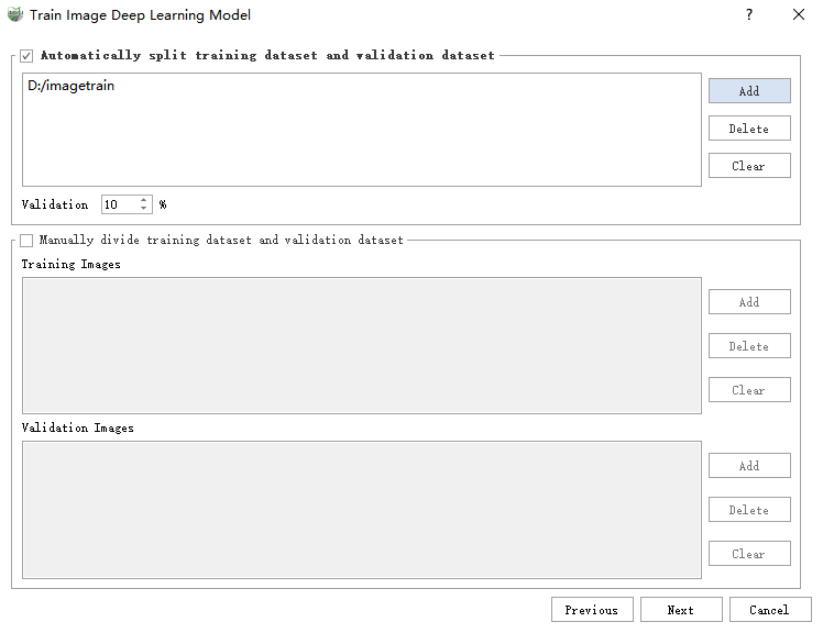
3) Click the Add button to add the annotated data folder from step 3, then click Next.

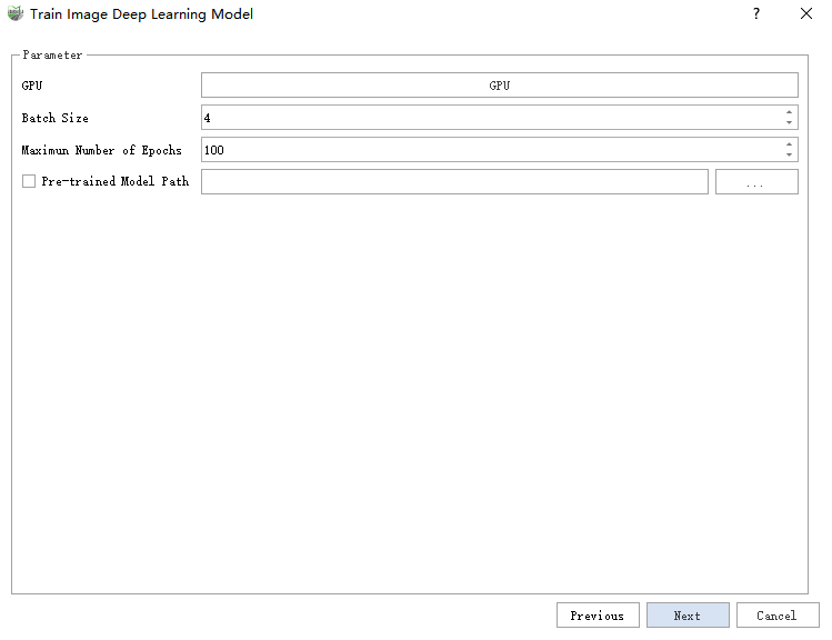
4) Set the parameters according to Train Image Deep Learning Model. In this example, select GPU, set batch size to 4, and train for 1000 epochs.

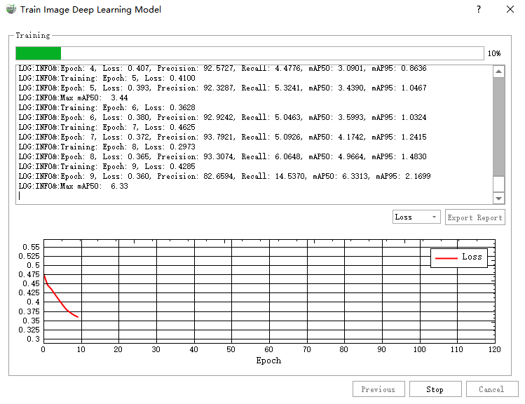
5) Click Next and then Start to begin training. This process takes a while and includes two stages. After the first progress bar reaches 100%, the second progress bar will start. Once training is complete, the result will look like this.

Training First Stage:

Training Second Stage:

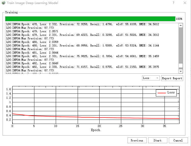
6) The loss curve has stabilized, indicating that the model has converged.

Loss Curve:

mAP50 Curve:

4.Inference

1) Click Raster -> Detect or Segment Object with Trained Model to open the inference interface. Select the image data and model trained in the previous step for inference.

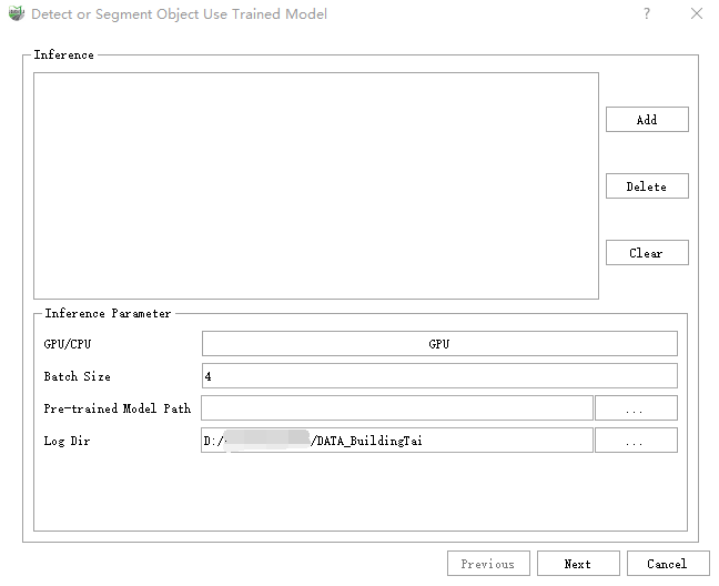
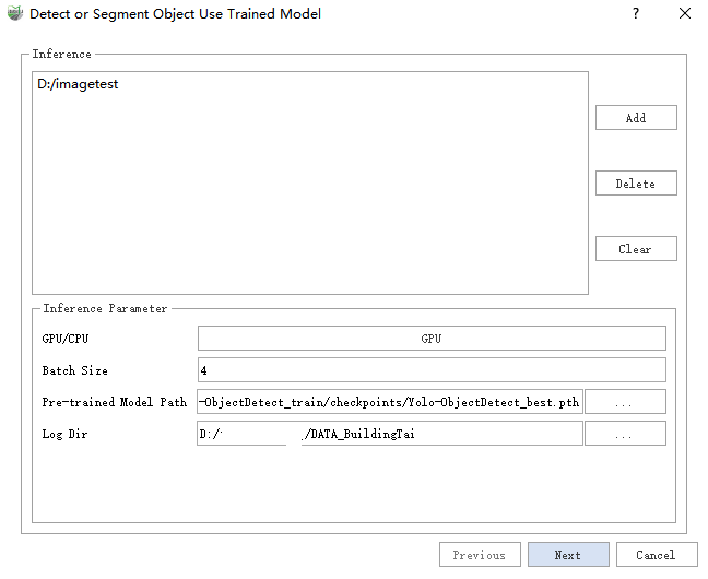
2) Click GPU to set whether to use GPU or CPU for inference.

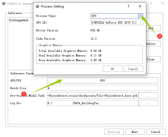
3) Set the batch size according to the GPU memory size, refer to Detect or Segment Target with Trained Model.

4) Click Next to go to the inference page.

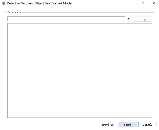
5) Click Start to begin inference. You can also click the stop button to interrupt inference.

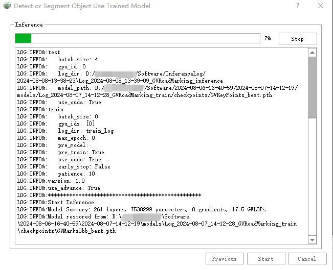
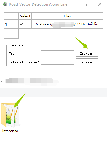
Once inference is complete, you can find the results in the inference directory under the same level as the data.

6)View Inference Results in the Annotation Tool

Open the inference folder, copy the latest inference file to the same directory as the images, then click Raster -> Start Labeling -> Open Dir, and select the inference folder to open and view.

7)Reproject to Point Cloud

For a detailed introduction to this function, refer to Road Vector.

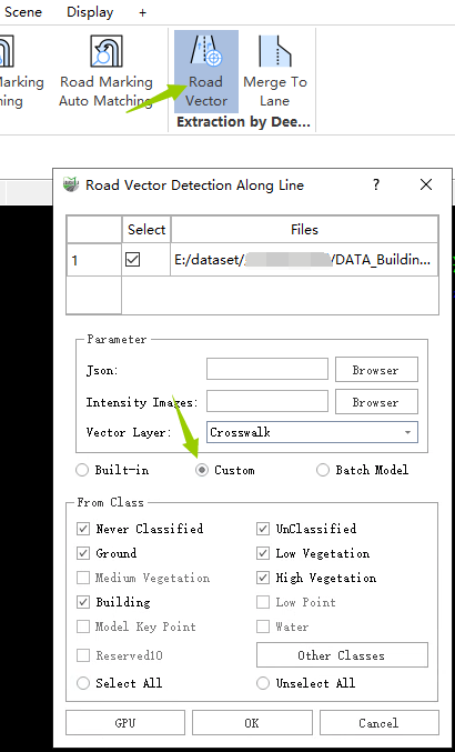
Click the Road Vector button under deep learning extraction in the Map Elements page, and select Custom mode.

Click the browse button for the Json parameter, and select the Json file obtained from inference. Click the browse button behind the intensity map, and select the intensity map path.

Select the class to project to the point cloud, such as ground points.

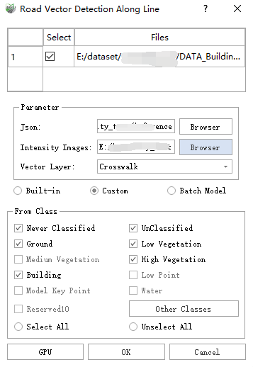
Project the extracted vectors onto the point cloud.