Fitting Geoid Model

Functional Overview

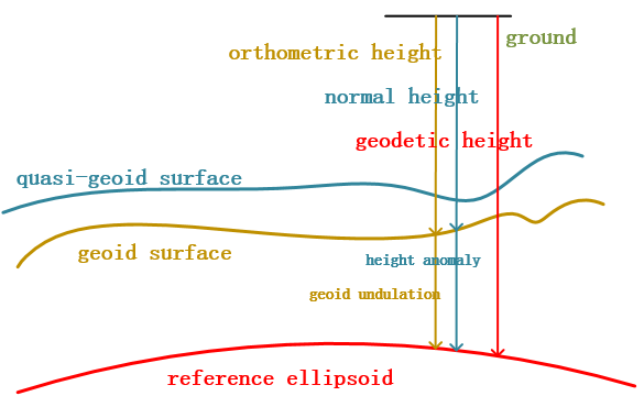
There are mainly three elevation datums involved in surveying: the physical surface of the earth - the geoidal surface, the mathematical surface of the earth - the reference ellipsoid, and an abstract geoid surface. These three elevation datums correspond to three commonly used elevation systems, namely: orthogonal, geodetic elevation and quasi-geodetic elevation system (normal elevation system). The relationship between these elevation datums is shown in the following figure. The elevation system currently used in China is the normal elevation system, while the GPS elevation is usually the geodetic elevation system. Since the reference ellipsoid does not coincide with the geoid, there is an elevation anomaly between the geodetic height and the normal height. The so-called GPS height fitting is the process of obtaining the abnormal height and then obtaining the normal height to establish a geoid surface. Analytical interpolation is the most commonly used method for elevation fitting. The main idea is to approximate the quasi-geoid with a curved surface to establish the closest quasi-geoid in the survey area, so as to calculate the elevation anomaly of any point in the survey area. But the analytical interpolation method requires that the height difference of the combined measurement points should not be too large, and the distance between the two points should not be too long, otherwise the terrain fluctuation between these points cannot be truly reflected.

The elevation fitting function mainly uses the geodetic height and normal height to solve the elevation anomaly process. LiDar360 currently supports four elevation fitting methods. They are plane fitting, linear interpolation, Conicoid fitting and cubic surface fitting. When choosing these mathematical models, first consider the distribution of GPS points (control points) and terrain conditions. Depending on the method and formula used, the minimum number of control points required for elevation fitting varies. These four methods all calculate the fitting parameters according to the least squares solution.

• Plane Fitting: At least 3 pairs of control points are required. The plane fitting method can be used in a small area or in a plain area to quickly obtain the required parameters with a small number of control points.
  • The plane fitting formula is ζ = a0 + a1x + a2y;
• Polynomial Curve Fitting. At least 4 pairs of control points are required. This method can be used if the GPS points are distributed in a line, and the geoid-like surface along the line is a continuous and smooth curve. But when using this method, the measured line should not be too long (usually controlled within 300 meters). If the fitting range is too large, the abnormal elevation changes of the points will be more complicated, and the resulting fitting errors will be larger.
  • The linear interpolation formula is ζ = a0 + a1x + a2x² + a3x³;
• Quadric Surface Fitting. At least 6 pairs of control points are required. In the small area GPS network, the geoid is regarded as Conicoid, and the elevation anomaly is expressed as a quadratic function of plane coordinates (x, y). The parameters are then fitted by least squares. Then each parameter is fitted by the least square method.
  • Conicoid fitting formula is ζ = a0 + a1x + a2y + a3xy + a4x² + a5y²;
• Trigonometric Fitting requires at least 10 pairs of control points. The principle is similar to Conicoid fitting, which expresses the elevation anomaly as a cubic function of plane coordinates (x, y).
  • The cubic surface fitting formula is ζ = a0 + a1x + a2y + a3xy + a4x² + a5y² + a6x²y + a7xy² + a8x³ + a9y³;

Usage

Click Data Management > Projection and Coordinate Conversion > Elevation Fitting

Parameters Settings

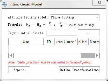
• Altitude Fitting Model: The four above-mentioned elevation fitting models can be selected from the drop-down menu. After you switch models, the formulas used by that model are also switched and displayed on the interface.
• Input Control Points: Import control point files in ascAll format. The control point file that needs to be selected must contain at least four columns, namely X, Y, geodetic height, and normal height. The imported control points will be displayed on the interface in the form of a table. The first column is "Whether it is a checkpoint". When this column is checked, the control point will be used for checking and not participating in the fitting. The number of control points involved in the fit must meet the minimum number of control points required for the elevation fit model. The control points participating in the fitting will be used to calculate the "inner coincidence accuracy", and the control points used for checking will be used to calculate the "outer coincidence accuracy". The same formula used for the accuracy of the inside and outside is: μ=√[VV]/(n-1) .
• Report: Use control points to perform elevation fitting and display the fitting results and accuracy assessments on the interface. The report can be saved in html format.
• Define Transformations: Use control points to perform elevation fitting and save the fitting results for next use. Refer to creating a transformation relationship.